Using Tableau to visualize land use change

Map of Land Use Categories by County. From the Tableau dashboard.

Map of Land Use Categories by County. From the Tableau dashboard.

I was home sick on Wednesday, so while I was on the couch I decided to dive into Tableau Public, a free desktop visualization tool. At IERP, we use Tableau for some of our public dashboards. Other than some minor playing around, I really did not use tool too much prior to this. It’s really great for working with complex data and seeing results quickly. Seeing that the 2012 Land Use data was released a few weeks ago, I wanted to see if I could bring it into PostgreSQL and produce some graphics of how the land use has changed over time.

View the Tableau Dashboard, the code to reproduce the data, and read on.

Continue reading

Posted in Data, Planning, PostgreSQL, Technology, Tools and Scripts, Visualization | Tagged , , , , , , | 1 Comment

Unix Philosophy

Often, when I go to tackle a problem, I look to use the simplest tools available first. Unix (and its derivatives/descendants, like Mac OS X and Linux) was designed with the following principles in mind:

Write programs that do one thing and do it well. Write programs to work together. Write programs to handle text streams, because that is a universal interface. —Doug McIlroy

One of my side projects is an index of property assessment records for New Jersey. The pages containing the property records all have the same URL structure:
/property/muncode/block/lot
Where the “muncode” is the 4 digit identifier for New Jersey municipalities published by the Division of Taxation, and the “block” and “lot” are the local level parcel identifiers. So each directory reflects essentially the spatial distribution of properties – lots will be near to other lots within the same block or municipal folder.

I recently wanted to see how each town was performing in terms of page views. Now, I can see such a report using the Content Drilldown in Google Analytics, but I really did not want to write something substantial to get at the information programmatically for further analysis.

Content Drilldown for NJParcels.com

Content Drilldown in Google Analytics


Content Drilldown is available through the API, so I could write something that authenticates against the API, performs the queries and stores the results, but that would be overkill, considering I also have the access log from Apache at my disposal.

I was able to make a report similar to what is on Google Analytics by using several Unix tools. Here’s what I did in one line to get the same type of information.

$ grep -oP '/property/\d+' access_log | sort | uniq -c | sort -rn
12289 /property/1508
11226 /property/0714
9630 /property/1506
8272 /property/0906
8130 /property/1507
...

First, grep (globally search with regular expressions and print) will take in a file – in this case, “access_log” – and return only the portion of each line that matches the regular expression/property/\d+“. The significant portion of that is the \d+ which means match one or more digits. Normally, grep returns the entire line when there is a match. The -oP are two flags to say only return the match and use Perl regular expressions.

If you’re not familiar with Unix, you may have once looked at your keyboard and thought, “what’s that vertical line and when would I ever need it?” The vertical line is often referred to as the “pipe” character, as it signifies that the output of one Unix tool should be passed (or piped) into the next tool written on the command line. With this, we can channel the results of a tool into the next tool for further processing.

The pipe character persists, even on an iPad keyboard.

The pipe character persists, even on an iPad keyboard.

We pipe the output of grep (a list of all second-order directories accessed by visitors) into sort. sort does what is sounds like, sorting each line returned alphabetically. We sort the output of grep to use the next tool to give us our count, uniq.

uniq collapses duplicate lines into one and can also provide a count of lines collapsed (using -c). In order for uniq to work properly, we need to sort the file first.

Finally, I sort the piped output one more time, now using the
r and n flags, which reverse the order and sort numerically instead of alphabetically, allowing me to see the most-visited municipalities at the top of my output.

I can further process these results, using other tools like awk and sed to perform other tasks, such as reformatting to CSV for loading into a database.

The Unix philosophy has always been in the back of my mind when working with Desktop GIS. The UIs are always so busy and complex that you often struggle with knowing what tool to use but being unable to find it. Or be stuck with the point-and-click mentality, where the tools expect human intervention in order to work. While concepts like ModelBuilder in ArcGIS Desktop are a step in the right direction, it still leaves much to be desired. Don’t get me wrong, I’m not suggesting we go back to AML, but we should put more thought into the tools that are available to us and use the ones that are best for the job. While I’m most at home programming in Python and could easily have written something in the language to parse the file and tally the results, it was ultimately much quicker to briefly experiment with existing tools and come up with a solution.

The right tools aren’t always the familiar ones, but you might become more familiar with them with some experimentation.

Posted in Data, Technology, Tools and Scripts | Comments Off on Unix Philosophy

Generating row and column IDs for a hexagon grid

hex_output

Recently when working on a project that uses a hexagon grid, I used the awesome mmqgis plugin to QGIS to produce the grid. The one small shortcoming with the tool is that I would prefer to have a cell identifier that is somehow related back to the position of the cell in the grid. I wanted an ID similar to a cartesian grid, specifying cells by row, then column. An integer “object id” wasn’t good enough.

The mmqgis plugin produces the grid according to your specifications as a shapefile in the current map projection. The plugin does not, for some reason, writes out an empty .prj file. I moved it into PostgreSQL using og2ogr and explicitly defined the projection (in this case, Web Mercator – 3857) while doing so.

$ ogr2ogr --config PG_USE_COPY YES 
    -f PGDump hex.sql hex.shp 
    -lco GEOMETRY_NAME=shape 
    -lco FID=objectid 
    -s_srs "EPSG:3857" 
    -t_srs "EPSG:3857”

I then began to work on creating my ID column. First, I would need to calculate a sequential number for both the row and the column.

ALTER TABLE hex ADD COLUMN rowid INT;
ALTER TABLE hex ADD COLUMN colid INT;

I would then need a sequence to generate the series of numbers used to count off the rows and columns.

CREATE TEMPORARY SEQUENCE idxid START WITH 1;

Now, I can use an update and a self-join to come up with a list of numbers for each column of hexagons. Hexagons are identified based on the integer value of the X coordinate of the cell’s center point. Joining the table to itself allows me to use the center points as the join criteria on a select distinct of centroid X values.

UPDATE hex SET colid = a.columnid
FROM (SELECT nextval('idxid') as columnid, b.centroidint
  FROM (SELECT DISTINCT ST_X(ST_CENTROID(shape))::int as centroidint 
    FROM hex 
    ORDER BY 1 ASC) b
  ) a
WHERE a.centroidint = ST_X(ST_CENTROID(shape))::int;

After calculating all of the column values, I restart the sequence and calculate the row values.

ALTER SEQUENCE idxid RESTART WITH 1;

UPDATE hex SET rowid = a.rowid
FROM (SELECT nextval('idxid') as rowid, b.centroidint
  FROM (SELECT DISTINCT ST_Y(ST_CENTROID(shape))::int as centroidint 
    FROM hex
    ORDER BY 1 ASC) b
  ) a
WHERE a.centroidint = ST_Y(ST_CENTROID(shape))::int;

Once I have a row and a column number for every cell, calculating the field is a straightforward update using concatenate.

ALTER TABLE hex ADD COLUMN hexid CHARACTER VARYING (10);
UPDATE hex SET hexid = 'r'||rowid::text||'c'||colid::text;

While writing this, I started to think about how I would go about doing this using ArcGIS. It was relatively quick to do – about 10 minutes from “I could use a different ID column” to the column being calculated. I am still not sure how I would do it using Arc. If you know a way to do this in ArcGIS, I’d love to hear about it – please leave a comment below.
You don’t have to do all of your GIS work in a database, but know that it can make life easier in many cases.

Posted in Data, PostgreSQL, Tools and Scripts | Tagged , , , , | Comments Off on Generating row and column IDs for a hexagon grid

“Doing more with SQL” talk at MAC URISA

Last week, I gave a 30 minute talk on “Doing More with SQL” at MAC URISA 2014. The slides from the talk are available below:

Continue reading

Posted in Conferences, PostgreSQL, Technology | Tagged , , , , , , , | 3 Comments

Insignificant Spaces

Yesterday, I mentioned that I discovered ArcGIS’s inconsistent handling of spaces within text fields. Today, I tested to see how ArcGIS handles NULLs, Empty Strings and Spaces within its native file formats.

Selecting 3 spaces selects all the strings.

Selecting 3 spaces selects all the strings.

Continue reading

Posted in Data, PostgreSQL, Technology, Tools and Scripts | Comments Off on Insignificant Spaces

Key issue with New Jersey’s parcel data

I’ve been working on a project to visualize differences between assessed value and levied taxes in New Jersey and I discovered a bug in some of New Jersey’s parcel data.

screenshot of ArcGIS with some incorrect parcels selected

256 parcels with the same PAMS_PIN key.

New Jersey uses “PAMS_PIN” as a key between the GIS data and the tax assessors’ rolls. The key is a simple concatenation: Municipal Code (a four digit value for each municipality), Block, and Lot joined by underscores. If the Qualifier Code (“QCODE”) field is populated, then that is also joined, again with an underscore. In Somerset County, many of these PAMS_PIN keys are incorrect, resulting in duplicates.

Continue reading

Posted in Data, Tools and Scripts | Comments Off on Key issue with New Jersey’s parcel data

Mitch Hedberg and GIS

So, a recent post on Reddit highlighted a Mitch Hedberg joke.

“La Quinta” is Spanish for “next to Denny’s.”

Thinking about this, I realized we could use GIS to find the number of La Quintas that are next to Denny’s. Last night after the kids were asleep, I sat down with a beer (Sierra Nevada) and figured out how I could get the data and perform the calculation.

First, I visited La Quinta’s website and their interactive map of hotel locations. Using Firebug, I found “hotelMarkers.js” which contains the locations of the chain’s hotels in JSON. Using a regular expression, I converted the hotel data into CSV.

A sample of the data, before and after conversion to CSV.

Sample of the data. Click for full size.

Next, I went to Denny’s website and their map. Denny’s uses Where2GetIt to provide their restaurant locations. They provide a web service to return an XML document containing the restaurants near the user’s location (via GeoIP) or by a specified address. Their web service also has a hard limit of 1,000 results returned per call. Again, I used Firebug to get the URL of the service, then changed the URL to search for locations near Washington, DC and Salt Lake City, Utah, with the result limit set to 1000 and the radius set to 10000 (miles, presumably). From this, I was able to get an “east” and “west” set of results for the whole country. These results were in XML, so I wrote a quick Python script to convert the XML to CSV.

#!/usr/bin/env python

import sys
from xml.dom.minidom import parse
dom = parse(sys.argv[1])
tags = ("uid", "address1", "address2", "city", "state", "country", "latitude", "longitude")
print ",".join(tags)
for poi in dom.getElementsByTagName("poi"):
    values = []
    for tag in tags:
        if len( poi.getElementsByTagName(tag)[0].childNodes ) == 1:
            values.append( poi.getElementsByTagName(tag)[0].firstChild.nodeValue )
        else:
            values.append("")
    print ",".join( map(lambda x: '"'+str(x)+'"', values) )

I then loaded the CSVs into PostgreSQL. First, I needed to remove the duplicates from my two Denny’s CSVs.

CREATE TABLE dennys2 (LIKE dennys);
INSERT INTO dennys2 SELECT DISTINCT * FROM dennys;
DROP TABLE dennys;
ALTER TABLE dennys2 RENAME TO dennys;

Then I added a Geometry column to both tables.

SELECT AddGeometryColumn('laquinta', 'shape', 4326, 'POINT', 2);
UPDATE laquinta SET shape = ST_SetSRID(ST_MakePoint(longitude, latitude),4326);
SELECT AddGeometryColumn('dennys', 'shape', 4326, 'POINT', 2);
UPDATE dennys SET shape = ST_SetSRID(ST_MakePoint(longitude, latitude),4326);

From there, finding all of the La Quinta hotels that live up to their name quite easy.

SELECT d.city, d.state, d.shape <-> l.shape as distance,
      ST_MakeLine(d.shape, l.shape) as shape
FROM dennys d, laquinta l 
WHERE (d.shape <-> l.shape) < 0.001 -- 'bout 100m
ORDER BY 3;

Here are the 29 cities that are home to La Quinta – Denny’s combos:

  • Mobile, AL
  • Phoenix, AZ
  • Bakersfield, Irvine, & Tulare, CA
  • Golden, CO
  • Orlando & Pensacola, FL
  • Augusta & Savannah, GA
  • Lenexa, KS
  • Metairie, LA
  • Amarillo, Austin, Brenham, College Station, Corpus Christi, Dallas, El Paso (2!), Galveston, Irving, Killeen, Laredo, Lubbock, McAllen, San Antonio, & The Woodlands, TX.

You might have noticed El Paso, Texas, has two La Quinta – Denny’s combos. Both happen to also be on the same street, just a few miles apart.

Gateway Boulevard to the West...

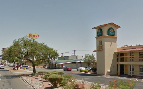
Gateway Boulevard to the West…
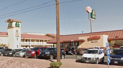
and further east on Gateway...

and further east…

I love that the second one even shares a post for both of their highway-scale signage.

So out of the 833 La Quintas and 1,675 Denny’s, there are 29 that are very close (if not adjacent) to one another. So, only 3.4% of the La Quintas out there live up to Mitch Hedberg’s expectations.

GIS: coming up with solutions for the problems no one asked!

Update: Chris in the comments made a good point about projection. So here’s the data reprojected into US National Atlas Equal Area and then limited to 150 meters distance between points.

SELECT d.city, d.state, ST_Transform(d.shape,2163) <-> ST_Transform(l.shape,2163) as distance 
FROM dennys d, laquinta l 
WHERE (ST_Transform(d.shape,2163) <-> ST_Transform(l.shape,2163)) < 150
ORDER BY 3;

This yields 49 pairs (or 5.8% of all La Quintas):

  • Alabama: Huntsville, Huntsville, Mobile
  • Arizona: Phoenix, Tempe, Tucson
  • California: Bakersfield, Bakersfield, Irvine, South San Francisco, Tulare
  • Colorado: Golden
  • Florida: Cocoa Beach, Orlando, Pensacola, St Petersburg
  • Georgia: Augusta, Savannah
  • Illinois: Schaumburg
  • Indiana: Greenwood
  • Kansas: Lenexa
  • Louisiana: Metairie
  • New Mexico: Albuquerque
  • Oregon: Salem
  • Texas: Amarillo, Austin, Brenham, College Station, Corpus Christi, Dallas, Dallas, El Paso, El Paso, Galveston, Irving, Killeen, Laredo, Live Oak, Lubbock, McAllen, San Antonio, San Antonio, San Antonio, Victoria, The Woodlands
  • Utah: Midvale
  • Virginia: Virginia Beach
  • Washington: Auburn, Seatac

This modification to the query introduced a new oddity: Huntsville, AL has a Denny’s that is between two La Quintas, which is why it’s on the revised list twice.

Between two La Quintas

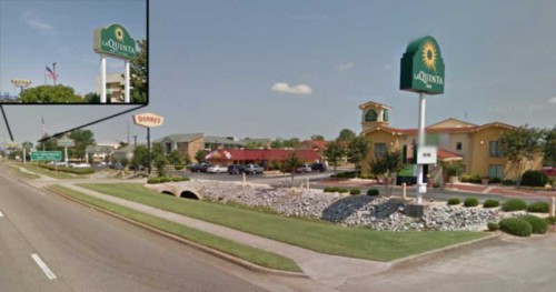
A Denny’s adjacent to one La Quinta and about 400 feet from another…

Update: I uploaded a dump of the data to Github, if you want to explore the data on your own.

Posted in Data, Google Maps, In the News, Teaching, Technology, Tools and Scripts, Web Mapping | 4 Comments

Using a TMS in JOSM’s Download Data window

Now that our crowdsourced update to New Jersey’s land use map has had some serious contributions – we’re just shy of 20,000 user-contributed points of new (2007-2012) urbanization – I realized that many of these locations are in need of updating in OpenStreetMap.

JOSM is my preferred editor for OpenStreetMap. I find it to be incredibly robust and powerful. I also love that it’s extensible; there are plenty of great plugins and it integrates with web services well. One thing that JOSM supports is WMS and TMS background imagery. I often use the freely-available 2012 imagery for New Jersey as a base for my edits. We’re also using the 2012 WMS for our NJ MAP “Growth” crowdsourcing web app to help identify areas of recent development in NJ. If you haven’t seen the app, check it out. It’s an easy to use app where 2012 imagery is presented along with a black mask derived from the 2007 urban lands in the Land Use/Land Cover data. Simply put, if you see a building on the aerials, click on it and tell us what it is.

Because those clusters of single family housing built post-2007 are not likely reflected in OpenStreetMap, I wanted to see if I could provide some base roadways for the new subdivisions as well as clean up the land use imported into OSM, which was from 2002.

I have a WMS service of the points in the Growth app, served up by GeoServer. GeoServer is also capable of providing the same data in TMS. While I was going to simply add a link to the WMS to JOSM, so that I could see the project’s contributions along side the aerial photo and the OSM data, I realized that it wouldn’t be as useful in the main map interface, because I’d only see the points after I downloaded some OSM data.

Screen Shot 2013-11-18 at 4.26.56 PM To help you find your area of interest, JOSM includes several OSM-derived map services  through the Download Data window. I did not realize that the list of layers included any TMS layers you added to JOSM. So instead of adding the new urban points from Growth as a WMS, I added them as a TMS. Now, instead of browsing for locations using Mapnik tiles, I can look for clusters of development points.

Screen Shot 2013-11-18 at 4.27.04 PMGranted, it’s not too meaningful – it’s just the points without any other background information – but it’s easy to find areas that likely need attention.

Screen Shot 2013-11-18 at 4.27.32 PMThis area was forest in 2002, but in 2012 is a new housing development. I was able to add the roads of the new development, as well as clean up the surrounding land use.

Screen Shot 2013-11-18 at 4.32.14 PMNow, I’ll still need to refer to another available source (such as NJ’s road network or our parcel data – both freely available under OSM-friendly licenses) for things like the road names, being able to focus in on areas that need updating in OSM will help us all improve the New Jersey portion of the world’s best free map.

If you want to help update OSM using NJ MAP: Growth as a guide, add the following TMS to JOSM:
tms:http://gis.rowan.edu:8080/geoserver/gwc/service/tms/1.0.0/njmap%3Acrowdsource_points@EPSG%3A900913@png/{zoom}/{x}/{-y}.png

Posted in Data, OpenStreetMap, Web Mapping | Tagged , , , , , , | Comments Off on Using a TMS in JOSM’s Download Data window

Portfolio Workshop

Yesterday, I held a Portfolio Workshop for our Rowan Geography and Environment students. The audio of my talk along with the slides are available on the workshop web page. While I think the talk and discussion was well-received, the audio is unedited, so you’ll hear plenty of ums and ahs before I hit my stride. I’ll probably repost this to YouTube with a clean narration at some later date.

Posted in Teaching | Tagged , , , , , | Comments Off on Portfolio Workshop

Rendering weirdness with reference data

Continued from yesterday’s post: Bizarre GeoServer WMS Rendering

Both the NJ Landscape Project habitat data and the Municipalities data are complex. It is hard to pinpoint a rendering issue when the data is very complex. I prepared a reference data set composed of a few multipart features. You can download the reference shapefile here.

Reference multipart polygons. Click for full size.

I created the polygon features in ArcGIS Desktop as a shapefile. I then imported the shapefile into my PostGIS database twice, once using PG_GEOMETRY & ArcSDE, the other using OGR. I then prepared two WMS layers in GeoServer, one based off of the SDE import and one from the OGR import. The SDE import causes GeoServer to improperly render the data. GeoServer can render the OGR import without issue.

Improperly rendered multipart features.

Improperly rendered multipart features.

I exported the geometries of each table as WKT: hexagons imported using SDE; hexagons imported using OGR. Note that the coordinates are essentially the same, but the “wrappers” around the coordinates are different. You can also tell that it is a rendering issue; in GeoServer’s layer preview mode, you can click on the OpenLayers map to identify a feature. Clicking on one of the erroneous polygons yields no results.

It appears that GeoServer is improperly handling MULTIPOLYGON features. POLYGON features (with multiple parts) are properly rendered. This is also what is being suggested in the support forum.

One other issue I encountered was that OGR would not import the shapefile without the -nlt flag set.

$ ogr2ogr -f "PostgreSQL" PG:"pg connection string" ./testing.shp -nln test_hexagons_ogr 
Warning 1: Geometry to be inserted is of type Multi Polygon, whereas the layer geometry type is Polygon.
Insertion is likely to fail
ERROR 1: INSERT command for new feature failed.
ERROR:  new row for relation "test_hexagons_ogr" violates check constraint "enforce_geotype_wkb_geometry"

Command: INSERT INTO "test_hexagons_ogr" ("wkb_geometry" , "id") VALUES ('snip'::GEOMETRY, 3) RETURNING "ogc_fid"
ERROR 1: Terminating translation prematurely after failed
translation of layer testing (use -skipfailures to skip errors)

$ ogr2ogr -f "PostgreSQL" PG:"pg connection string" ./testing.shp -nln test_hexagons_ogr -nlt POLYGON
$
Posted in Data, Web Mapping | Tagged , , | 5 Comments